Tutorials

Tutorial 1: Reference based particle picking

In this tutorial we describe how to use TomoTwin for picking in tomograms using references.

Note

Example Dataset

To check if everything is working you can use our demo for EMPIAR 10499. As for this demo the pixel size is already reasonable, you can skip step 1 of the tutorial. The folder reference_output contains the results when we run it locally. The file run.sh contains all commands we run. The total runtime was ~ 30 minutes on 2 x A100 GPUs.

Download: https

1. Rescale your Tomogram

TomoTwin has been trained on tomograms with a pixel size of 10Å. While in practice we’ve used it with pixel sizes ranging from 9.2Å to 25.0Å, it’s probably often ideal to run it with a pixel size close to 10Å. However, for proteins equal to or larger than the ribosome, we have found that a larger pixel size (e.g. 15Å) works better. For this you may need to rescale your tomogram. You can do this by Fourier shrinking your tomogram with EMAN2. Suppose you have a tomogram with a pixel size of 5.9359Å. The Fourier shrink factor is then 10Å/5.9359Å = 1.684

e2proc3d.py --apix=5.9359 --fouriershrink=1.684 your_tomo.mrc your_tomo_a10.mrc

TomoTwin should be used to pick on tomograms without denoising or lowpass filtering. But you may use these tomograms to find the coordinates of your particle of interest for use as a reference. In this case, you should make sure the denoised/lowpass filtered tomogram has the same pixel size as the one you will pick on.

What if my protein is too big for a box size of 37x37x37 pixels?

Because TomoTwin was trained on many proteins at once, we needed to find a box size that worked for all proteins. Therefore, all proteins were used with a pixel size of 10Å and a box size of 37 pixels. Because of this, you must extract your reference with a box size of 37 pixels. If your protein is too large for ths box at 10Å/pix (much larger than a ribosome) then you should scale the pixel size of your tomogram until it fits rather than changing the box size. Likewise if your protein is so small that at 10Å/pix it only fills one to two pixels of the box, you should scale your tomogram pixel size until the particle is bigger, however we’ve found that for proteins down to 100 kDa, 10Å/pix is sufficient for the 37 box.

2. Pick and extract your reference

For the reference based approach you need, of course, references. To pick them follow the next steps:

1. Open your tomogram in napari

Note

For easy identification of your reference particle we recommend to use low-pass filter to 60Å and/or denoising (be sure it has the same pixel size of the tomogram you will pick on).

napari_boxmanager your_tomo_a10.mrc

2. Select organize_layer tab of the boxmanager toolkit (lower right corner). Press the button Create particle layer.

3. Switch to the boxmanager tab and set the boxsize to 37, as this gonna be the box size we will use for extraction later on.

4. Identify a potential reference, choose the slice so that its centered and pick it by clicking in the center of the particle. Continue doing that until you think you have enough references

Note

Use multiple references per particle class

We recommend to pick multiple (3-4) references per protein of interest, as not all subvolumes work equally well.

Each reference can be later evaluated separately using the boxmanager, allowing you to decide which gives the best result for each protein of interest

5. Optional: If you want to pick another protein class, we recommend to create a separate particle layer for it (step 2).

6. To save the reference of the selected particle layer (see layer list in napari), click on File -> Save Selected Layer(s). Create a new folder by right click in the dialog and name it for example ‘coords’. Now select as Files of type the entry Box Manager. Use the filename reference.coords and press Save.

7. Finally, use the tomotwin_tools.py extractref script to extract a subvolume from the tomogram (the original, not the denoised / low pass filtered) at the coordinates for each reference. If there are multiple references you would like to pick in the tomogram, repeat this process multiple times giving a new output folder each time.

tomotwin_tools.py extractref --tomo tomo/your_tomo_a10.mrc --coords path/to/references.coords --out reference/ --filename protein_a

You will find your extracted references in reference/protein_a_X.mrc where X is a running number.

3. Embed your Tomogram

I assume that you already have downloaded the general model.

To embed your tomogram using two GPUs and batchsize of 256 use:

CUDA_VISIBLE_DEVICES=0,1 tomotwin_embed.py tomogram -m LATEST_TOMOTWIN_MODEL.pth -v your_tomo_a10.mrc -b 256 -o out/embed/tomo/ -s 2

Hint

The batchsize parameter

To have your tomograms embedded as quick as possible, you should choose a batchsize that utilize your GPU memory as much as possible. However, if you choose it too big, you might run into memory problems. In those cases play around with different batch sizes and check the memory usage with nvidia-smi.

Hint

Strategy: Speed up embedding calculation using a mask

Using masks can dramatically speed up the embedding calculation. It can also improve the estimated umaps!

Check out the corresponding strategy!

4. Embed your reference

Now you can embed your reference:

CUDA_VISIBLE_DEVICES=0,1 tomotwin_embed.py subvolumes -m LATEST_TOMOTWIN_MODEL.pth -v reference/*.mrc -b 12 -o out/embed/reference/

Hint

Strategy: Refine your reference using umaps

Some references just don’t work well - you can try to refine it using umaps.

Check out the corresponding strategy!

5. Map your tomogram

The map command will calculate the pairwise distances/similarity between the references and the subvolumes and generate a localization map:

tomotwin_map.py distance -r out/embed/reference/embeddings.temb -v out/embed/tomo/your_tomo_a10_embeddings.temb -o out/map/

6. Localize potential particles

To locate potential particles positions for each target run:

tomotwin_locate.py findmax -m out/map/map.tmap -o out/locate/

Hint

Similarity maps

You can add the option --write_heatmaps to the locate command. If you do this you will find a similarity map for each reference in your_tomo_a10/locate/ - just in case you are interested, this is akin to a location confidence heatmap for each protein.

7. Inspect your particles with the boxmanager

Open your particles with the following command or drag the files into an open napari window:

napari_boxmanager tomo/your_tomo_a10.mrc out/locate/located.tloc

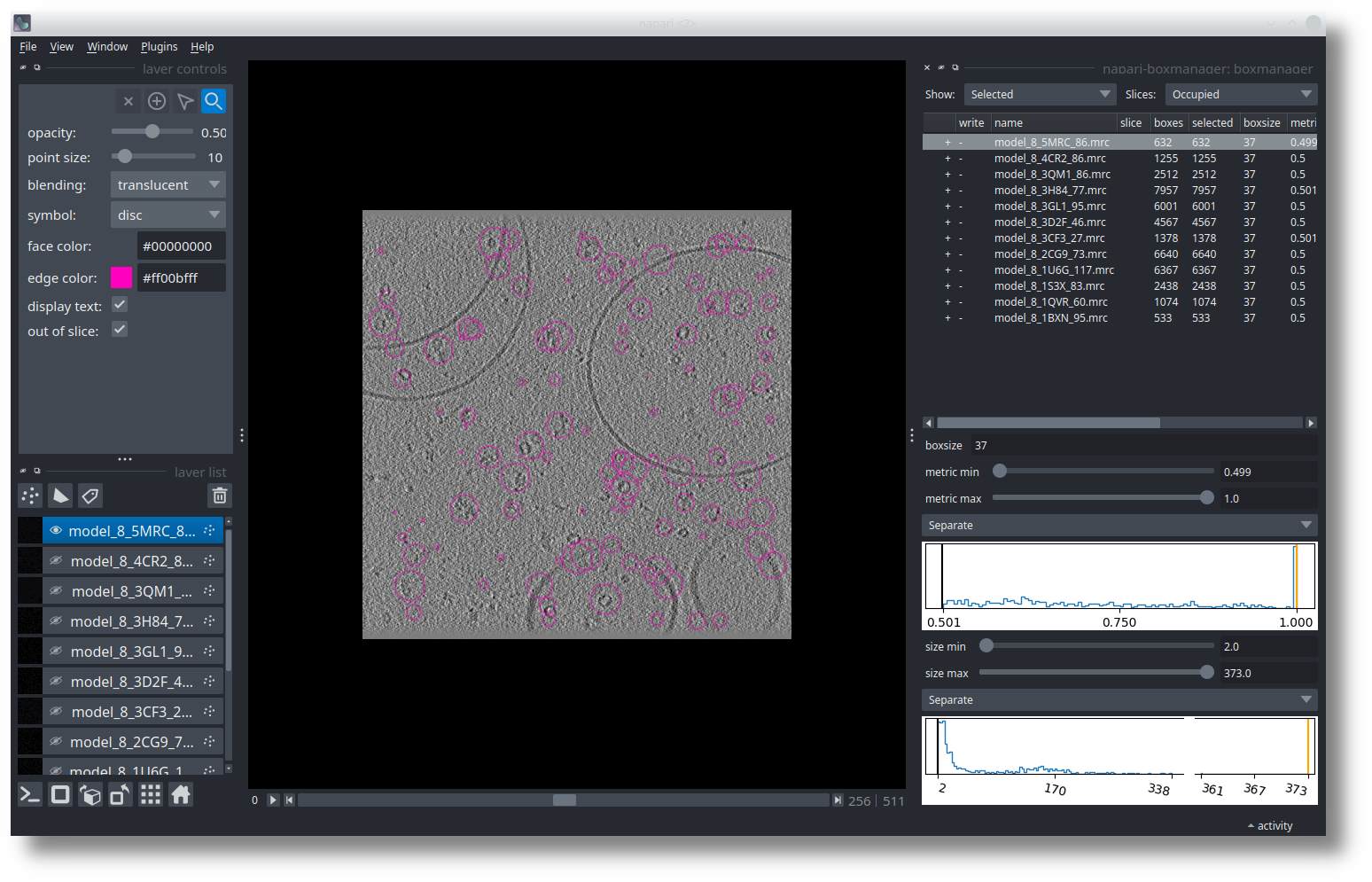
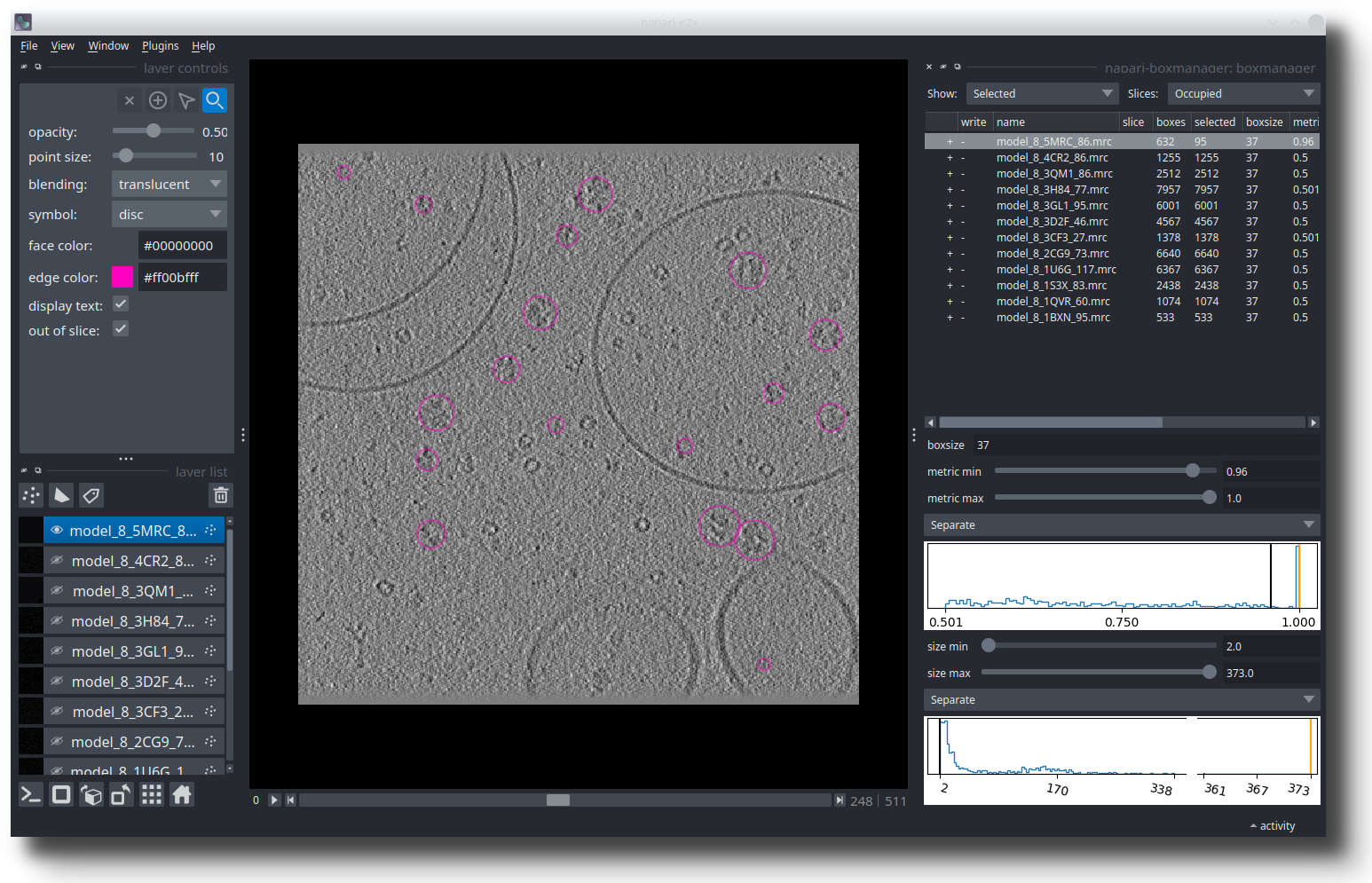
The example shown here is from the SHREC competition. In the table on the right you see 12 references. I selected the model_8_5MRC_86.mrc, which is a ribosome. Below the table, you need to adjust the metric min and size min thresholds until you like the results. After the optimization is done the result might look similar to this:

In the left panel, select the references you would like to pick (Control + LMB on linux/windows, CMD + LMB on mac to select multiple). You can now press File -> Save selected Layer(s). In the dialog, change the Files of type to Box Manager. Choose filename like selected_coords.tloc. Make sure that the file ending is .tloc.

To convert the .tloc file into .coords you need to run

tomotwin_pick.py -l coords.tloc -o coords/

You will find coordinate file for each reference in .coords format in the coords/ folder.

Hint

Strategy: Improve your picks by refining your references

Manual selected references can sometimes be optimized using umaps!

Check out the corresponding strategy!

8. Scale your coordinates

After step 7 you have the coordinates for each protein of interest in your tomogram. Assuming you downscaled your tomogram in step 1, you now need to scale your coordinates to the pixel size you would like to use for extraction. Assuming that you would like to extract from tomograms with a pixel size of 5.936 A/pix, then the command would be:

tomotwin_tools.py scale_coordinates --coords coords/your_coords_file.coords --tomotwin_pixel_size 10 --extraction_pixel_size 5.9356 --out multi_refs_0_a5936.coords

Tutorial 2: Clustering based particle picking

1. Rescale your Tomogram

TomoTwin has been trained on tomograms with a pixel size of 10Å. While in practice we’ve used it with pixel sizes ranging from 9.2Å to 25.0Å, it’s probably often ideal to run it with a pixel size close to 10Å. However, for proteins equal to or larger than the ribosome, we have found that a larger pixel size (e.g. 15Å) works better. For this you may need to rescale your tomogram. You can do this by Fourier shrinking your tomogram with EMAN2. Suppose you have a tomogram with a pixel size of 5.9359Å. The Fourier shrink factor is then 10Å/5.9359Å = 1.684

e2proc3d.py --apix=5.9359 --fouriershrink=1.684 your_tomo.mrc your_tomo_a10.mrc

TomoTwin should be used to pick on tomograms without denoising or lowpass filtering. But you may use these tomograms for visualizing the picks in Napari. In this case, you should make sure the denoised/lowpass filtered tomogram has the same pixel size as the one you will pick on (downscaling it if necessary).

What if my protein is too big for a box size of 37x37x37 pixels?

Because TomoTwin was trained on many proteins at once, we needed to find a box size that worked for all proteins. Therefore, all proteins were used with a pixel size of 10Å and a box size of 37 pixels. Because of this, you must extract your reference with a box size of 37 pixels. If your protein is too large for ths box at 10Å/pix (much larger than a ribosome) then you should scale the pixel size of your tomogram until it fits rather than changing the box size. Likewise if your protein is so small that at 10Å/pix it only fills one to two pixels of the box, you should scale your tomogram pixel size until the particle is bigger, however we’ve found that for proteins down to 100 kDa, 10Å/pix is sufficient for the 37 box.

2. Embed your Tomogram

I assume that you already have downloaded the general model.

To embed your tomogram using two GPUs and batchsize of 256 use:

CUDA_VISIBLE_DEVICES=0,1 tomotwin_embed.py tomogram -m LATEST_TOMOTWIN_MODEL.pth -v your_tomo_a10.mrc -b 256 -o out/embed/tomo/ -s 2

Hint

The batchsize parameter

To have your tomograms embedded as quick as possible, you should choose a batchsize that utilize your GPU memory as much as possible. However, if you choose it too big, you might run into memory problems. In those cases play around with different batch sizes and check the memory usage with nvidia-smi.

Hint

Strategy: Speed up embedding calculation using a mask

Using masks can dramatically speed up the embedding calculation. It can also improve the estimated umaps!

Check out the corresponding strategy!

3. Estimate UMAP manifold and Generate Embedding Mask

Now we will approximate the tomogram embeddings to 2D to allow for efficient visualization. To calculate a UMAP:

tomotwin_tools.py umap -i out/embed/tomo/tomo_embeddings.temb -o out/clustering/

Note

If you encounter an out of memory error here, you may need to reduce the fit_sample_size and/or chunk_size values (default 400,000).

4. Load data for clustering in Napari

Now that we have all the input files for the clustering workflow we can get started in Napari. First open your tomogram and the embedding mask by:

napari your_tomo_a10.mrc

Next open the napari-tomotwin clustering tool via Plugins -> TomoTwin clustering workflow. Then choose the Path to UMAP by clicking on Select file and provide the path to your your_tomo_a10_embeddings.tumap. Click Load and a 2D plot of the umap embeddings should appear in the plugin window. It will do some calculating in the background and might take a few seconds.

5. Find target cluster

Once you loaded a umap by the previous step, a set of tools will open.

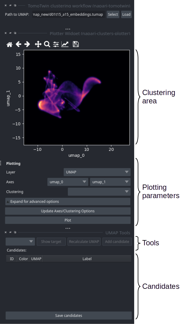
• Clustering area: Here you can select clusters within the umap using the lasso (freehand) tool.

• Plotting parameters: Only two options are relevant for TomoTwin. The Layer combo box allows you to select which UMAP you want to visualize. At the beginning only one UMAP is available. Later in the workflow, more may appear. If you change it, you need to press the Plot button to update the UMAP. The second relevant option is the Log scale plot. For this you need to expand the advanced options and check the log scale checkbox.

• Tools: Here you will find some helpful tools. First you need to select a cluster from the dropdown box. Show target will help you evaluate if a cluster might be a good target. Recompute UMAP allows you to refine a selected cluster. Once you have found a good cluster, you can add it to the candidate list with Add candidate.

• Candidates: Each row represents a candidate target. The labels are label changeable. Left clicking on the table allows to Show or the Delete a candidate. Sve the candidate targets to disk by pressing Save candidates.

Use log scale to see weak clusters

When the abundance of the protein is low, the clusters are often difficult to detect. Using a log scale for the plot may show clusters that are otherwise difficult to spot. To activate the log scale click on Advanced settings Log scale.

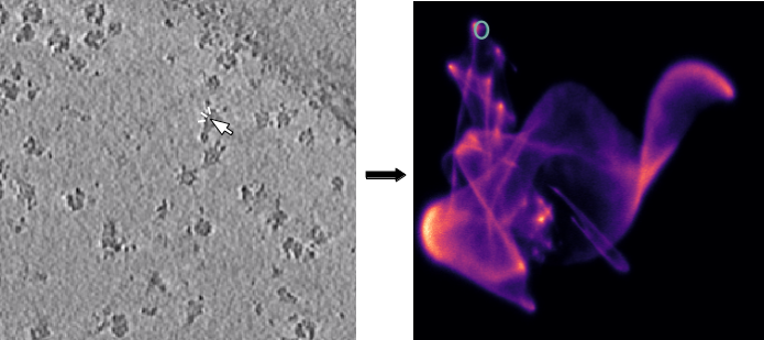
Locate potential targets

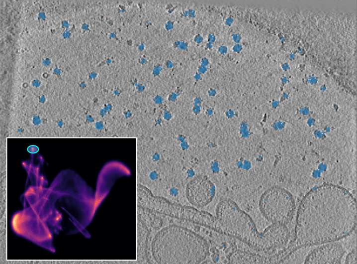
The next step is to generate potential targets from the 2D umap. We will use a tomogram that shows two distinct particle populations (yellow: Tc toxin, blue: ribosome) as example:

Tomogram with UMAP inset. Two quite distinct particle populations can be identified. The yellow circle highlights a toxin particle, the blue circle a ribosome particle.

You can use the interactive lasso (freehand) tool from the “napari cluster plotter” to select clusters in the UMAP. When you outline an area in the UMAP, the corresponding area in the tomogram is highlighted.

Tomogram with UMAP as inset. The selected cluster contains both particle populations.

The Anchor tool helps to locate clusters in the UMAP

Clicking on the tomogram creates an “anchor” (a little circle) in the UMAP. The anchor can help you to locate a cluster in the UMAP. By holding Shift you can add multiple anchors.

Refine cluster targets

The selection we made is not satisfactory as both the toxins and the ribosomes are selected. TomoTwin uses UMAPs to reduce the 32-dimensional embedding space to a 2-dimensional space that can be visualized. However, this reduction is not perfect and sometimes a cluster can actually contain several sub-clusters. Pressing Recompute UMAP will compute a new UMAP for the embeddings contained in the selected cluster.

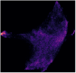
Recalculated UMAP for the embeddings contained in the previously selected cluster.

The new umap shows new structure. If we select the rather densely populated area on the left, we have identified the cluster that exclusively represents the toxin cluster. To select the ribosome cluster, we lasso the tip of the larger and fuzzier area by holding Shift while outlining the area.

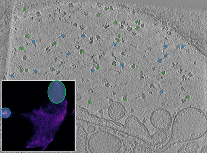
In the recalculated UMAP we can now separate the toxin from the ribosome cluster.

For the ribosome, we could get a more “complete” highlighting if we had selected the entire area. However, the way we did it is preferable because we only get the center of the ribosome, which results in better centered picks.

As a sanity check, we can press Show target for each cluster in the dropdown list. In TomoTwin, a cluster is reduced and represented by a single embedding point (the cluster center). It is a good sanity check to visualize which of the points in your cluster represents your cluster. By clicking Show target, the center (medoid) is calculated and visualized in the tomogram by a circle in the cluster color. If the circle is roughly centered on your protein of interest, its probably a good target. If the circle is approximately centered on your protein of interest, it is probably a good target. If it is not centered on a target, but rather on background, other structures or contamination, you should continue to refine your cluster target. Here, both cases are centered on the toxin and ribosome, respectively.

Add and save candidates

Now that we are satisfied with our selection, we can add both clusters to the candidate list by selecting each cluster in the drop-down list and pressing Add candidate.

We recommend that you change the label of each candidate by double-clicking with the left mouse button in one of the label cells.

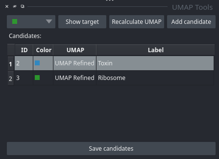
All potential targets are listed and labeled candidates table. Right click on a row allow to Delete the candidate or by pressing Show to restore the UMAP selection.

Finally, we can save the the corresponding labels to disk by pressing Save candidates. Select a folder and write the candidate to disk. The folder will contain several files:

• cluster_targets.temb: This is the file you will use in the next steps. It contains the medoid embedding for each cluster.

• embeddings_CLUSTER_LABEL.temb: One file per cluster. It contains all the embeddings that are part of that cluster.

• medoid_CLUSTER_LABEL.coords: The coordinates of the cluster centre (medoid). This is the same as what you get when you click on Show target

Check out the video demo of selecting clusters

6. Map your tomogram

The map command will calculate the pairwise distances/similarity between the targets and the tomogram subvolumes and generate a localization map:

tomotwin_map.py distance -r out/clustering/cluster_targets.temb -v out/embed/tomo/your_tomo_a10_embeddings.temb -o out/map/

7. Localize potential particles

To locate potential particles positions for each target run:

tomotwin_locate.py findmax -m out/map/map.tmap -o out/locate/

Hint

Similarity maps

You can add the option --write_heatmaps to the locate command. If you do this you will find a similarity map for each reference in your_tomo_a10/locate/ - just in case you are interested, this is akin to a location confidence heatmap for each protein.

Open your particles with the following command or drag the files into an open napari window:

napari_boxmanager tomo/your_tomo_a10.mrc out/locate/located.tloc

The example shown here is from the SHREC competition. In the table on the right you see 12 references. I selected the model_8_5MRC_86.mrc, which is a ribosome. Below the table, you need to adjust the metric min and size min thresholds until you like the results. After the optimization is done the result might look similar to this:

In the left panel, select the references you would like to pick (Control + LMB on linux/windows, CMD + LMB on mac to select multiple). You can now press File -> Save selected Layer(s). In the dialog, change the Files of type to Box Manager. Choose filename like selected_coords.tloc. Make sure that the file ending is .tloc.

Hint

Strategy: Improve your picks by refining your cluster targets

Cluster targets can sometimes be optimized using umaps!

Check out the corresponding strategy!

To convert the .tloc file into .coords you need to run

tomotwin_pick.py -l coords.tloc -o coords/

You will find coordinate file for each reference in .coords format in the coords/ folder.

8. Scale your coordinates

After step 7 you have the coordinates for each protein of interest in your tomogram. Assuming you downscaled your tomogram in step 1, you now need to scale your coordinates to the pixel size you would like to use for extraction. Assuming that you would like to extract from tomograms with a pixel size of 5.936 A/pix, then the command would be:

tomotwin_tools.py scale_coordinates --coords coords/your_coords_file.coords --tomotwin_pixel_size 10 --extraction_pixel_size 5.9356 --out multi_refs_0_a5936.coords